June 28, 2024/
Linkedin Instagram Facebook X-twitter Case Study Automating the generation of javascript expressions with Pre-Trained AI Models Challenge Developing a user-friendly…


As Tech Co-Founder at Yugensys, I’m passionate about fostering innovation and propelling technological progress. By harnessing the power of cutting-edge solutions, I lead our team in delivering transformative IT services and Outsourced Product Development. My expertise lies in leveraging technology to empower businesses and ensure their success within the dynamic digital landscape.
Looking to augment your software engineering team with a team dedicated to impactful solutions and continuous advancement, feel free to connect with me. Yugensys can be your trusted partner in navigating the ever-evolving technological landscape.
Linkedin Instagram Facebook X-twitter Case Study Automating the generation of javascript expressions with Pre-Trained AI Models Challenge Developing a user-friendly…
Linkedin Instagram Facebook X-twitter In today’s tech landscape, harnessing the capabilities of artificial intelligence (AI) is pivotal for creating innovative…

Linkedin Instagram Facebook X-twitter Welcome to our comprehensive guide on bundling a React library into a reusable component library! In…
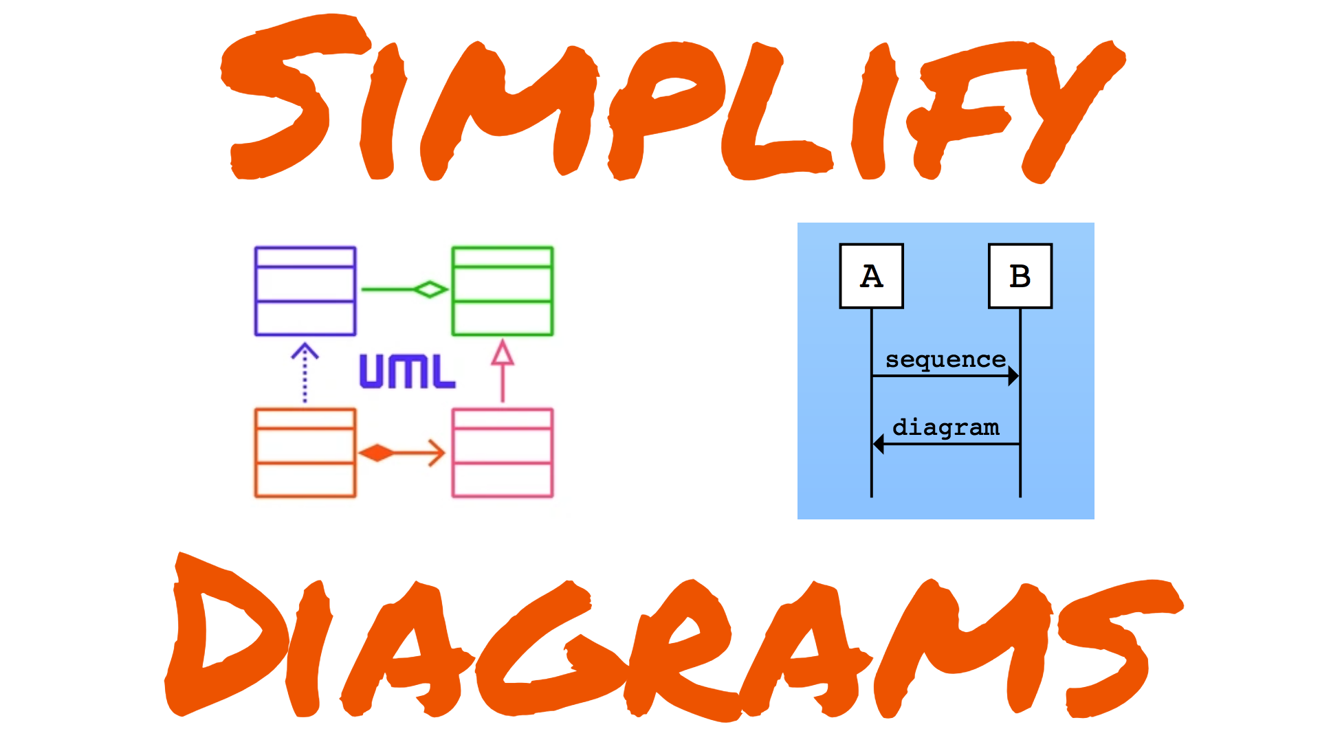
Linkedin Instagram Facebook X-twitter In today’s tutorial, we’ll explore creation of stunning diagrams using ChatGPT, along with the assistance of…