Bayesian Machine Learning Explained: A Probabilistic Approach to Data Modeling
Table of Contents
Introduction
Bayesian Machine Learning is a powerful and flexible approach that uses probability theory to model uncertainty in machine learning. Unlike frequentist methods that provide point estimates for parameters, Bayesian methods treat parameters as random variables with their own distributions. This allows us to incorporate prior knowledge and update our beliefs as new data becomes available.
Fundamental Concepts
1. Bayes' Theorem
Bayes’ Theorem is the cornerstone of Bayesian inference. It relates the conditional and marginal probabilities of random events. Mathematically, it is expressed as:
\[P(\theta \mid D) = \frac{P(D \mid \theta) \cdot P(\theta)}{P(D)}\]
where:
• \(\theta\) represents the model parameters.
• \(D\) represents the observed data.
• \(P(\theta \mid D)\) is the posterior probability, the probability of the parameters given the data.
• \(P(D \mid \theta)\) is the likelihood, the probability of the data given the parameters.
• \(P(\theta)\) is the prior probability, the initial belief about the parameters.
• \(P(D)\) is the marginal likelihood or evidence, the total probability of the data.
2. Priors
3. Likelihood
The likelihood function \(P(D | \theta)\) represents the probability of observing the data given the parameters. For instance, if our data follows a normal distribution:
\[ D_i \sim \mathcal{N}(\theta, \sigma^2) \]
the likelihood for a dataset
\[ P(D | \theta) = \prod_{i=1}^n \mathcal{N}(D_i | \theta, \sigma^2) \]
4. Posterior
The posterior distribution \(P(\theta \mid D)\) combines the prior and the likelihood to update our belief about the parameters after observing the data. This is obtained through Bayes’ Theorem.
5. Marginal Likelihood
Bayesian Inference
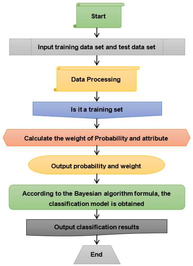
Bayesian inference involves calculating the posterior distribution given the prior and likelihood. This process can be computationally intensive, often requiring approximation methods.
We can represent the knowledge as:
- \(F_{i,j}\): Cell \(C_{i,j}\) is free.
- \(B_{i,j}\): Cell \(C_{i,j}\) is blocked.
The robot’s knowledge base (KB) includes the following rules:
- If a cell \(C_{i,j}\) is blocked, then the robot cannot move into that cell: \(Bi,j→¬Fi,j\).
- If the robot perceives no obstacles in adjacent cells, it can safely move forward.
1. Conjugate Priors
Conjugate priors simplify Bayesian updating. A prior \(P(\theta)\) is conjugate to the likelihood \(P(D \mid \theta)\) if the posterior \(P(\theta \mid D)\) is in the same family as the prior. For example, for a Gaussian likelihood with known variance:
\[ D_i \sim \mathcal(\theta, \sigma^2) \]
\[ \theta \sim \mathcal{N}(\mu_0, \sigma_0^2) \]
The posterior is also Gaussian:
\[ \theta | D \sim \mathcal{N}(\mu_n, \sigma_n^2) \]
where:
\[ \sigma_n^2 = \left( \frac{1}{\sigma_0^2} + \frac{n}{\sigma^2} \right)^{-1} \]
\[ \mu_n = \sigma_n^2 \left( \frac{\mu_0}{\sigma_0^2} + \frac{\sum_{i=1}^n D_i}{\sigma^2} \right) \]
2. Markov Chain Monte Carlo (MCMC)
When conjugate priors are not available, we use numerical methods like MCMC to approximate the posterior distribution. MCMC generates samples from the posterior, which can be used to estimate expectations and variances.
Popular MCMC algorithms include:
• Metropolis-Hastings : Generates a Markov chain using a proposal distribution and acceptance criteria.
• Gibbs Sampling : Iteratively samples from conditional distributions.
Use Cases and Benefits
Bayesian methods are widely used in various applications due to their flexibility and ability to incorporate uncertainty and prior knowledge.
1. Medical Diagnostics
Use Case: Predicting the probability of a disease given symptoms and medical history.
Benefit: Bayesian methods allow incorporating prior medical knowledge and patient history, providing more personalized and accurate predictions.
For example, in diagnosing a condition \(P(C)\) given symptoms and test results \(P(S,T)\) :
\[ P(C | S, T) = \frac{P(S, T | C) P(C)}{P(S, T)} \]
2. Financial Forecasting
Use Case: Predicting stock prices or economic indicators.
Benefit: Bayesian methods can update predictions as new data becomes available, adapting to market changes.
For instance, predicting stock price given historical data \(P(P \mid D)\):
\[ P(P | D) = \int P(P | \theta) P(\theta | D) d\theta \]

3. Natural Language Processing / Computer Vision
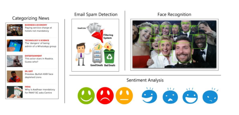
Use Case: Text classification, Categorizing News, Email Spam Detection, Face Recognition and Sentiment Analysis.
Benefit: Bayesian methods, such as Naive Bayes, handle sparse data well and provide probabilistic interpretations of classifications.
The general form of the Naive Bayes conditional independence assumption can be expressed mathematically as:
\[
P(C | X_1, X_2, \ldots, X_n) = \frac{P(C) \cdot \prod_{i=1}^{n} P(X_i | C)}{P(X_1, X_2, \ldots, X_n)}
\]
Here:
- \(P(C|X_1,X_2,\ldots,X_n)\) is the posterior probability of class \(C\) given the features \(X_1,X_2,\ldots,X_n\).
- \(P(C)\) is the prior probability of class \(C\).
- \(P(X_i|C)\) is the likelihood of feature \(X_i\) given class \(C\).
- \(P(X_1,X_2,\ldots,X_n)\) is the marginal probability of observing the features \(X_1,X_2,\ldots,X_n\).
The product operator \(\prod_{i=1}^n\) indicates that you multiply the likelihoods of the individual features given the class CCC. This is a key part of the Naive Bayes assumption, which assumes that the features are conditionally independent given the class.
In simpler terms, the symbol “\(\prod\)” in this context tells you to take the product of the probabilities of each feature \(X_i\) occurring given the class \(C\), and this product is then combined with the prior probability of the class CCC to compute the posterior probability.
4. Robotics
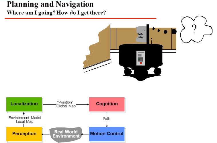
Use Case: Path planning and localization.
Benefit: Bayesian methods can model the uncertainty in sensor data and the environment, leading to more robust decision-making.
For example, estimating the robot’s position given sensor readings \(P(X \mid S)\):
\[ P(X | S) = \frac{P(S | X) P(X)}{P(S)} \]
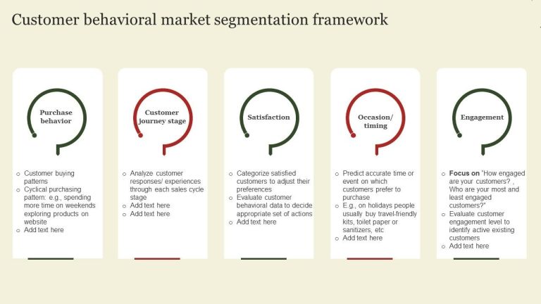
5. Marketing and Customer Segmentation
Use Case: Predicting customer behavior and segmenting markets.
Benefit: Bayesian methods can incorporate prior market knowledge and continuously update segmentation models as new data is collected.
For example, segmenting customers based on purchase history \(P(C \mid H)\):
\[ P(C | H) = \frac{P(H | C) P(C)}{P(H)} \]
Conclusion
Bayesian Machine Learning offers a robust framework for incorporating uncertainty and prior knowledge into machine learning models. By leveraging probabilistic methods, Bayesian approaches provide a more nuanced understanding of model parameters and their distributions, leading to better decision-making and more interpretable results.
Bayesian methods, while computationally intensive, offer significant advantages, especially in scenarios where uncertainty is paramount. As computational resources and algorithms improve, the application of Bayesian techniques is likely to become more prevalent in the machine learning community. The ability to continuously update models with new data and incorporate prior knowledge makes Bayesian Machine Learning a valuable tool for a wide range of applications.
As the Tech Co-Founder at Yugensys, I’m driven by a deep belief that technology is most powerful when it creates real, measurable impact.
At Yugensys, I lead our efforts in engineering intelligence into every layer of software development — from concept to code, and from data to decision.
With a focus on AI-driven innovation, product engineering, and digital transformation, my work revolves around helping global enterprises and startups accelerate growth through technology that truly performs.
Over the years, I’ve had the privilege of building and scaling teams that don’t just develop products — they craft solutions with purpose, precision, and performance.Our mission is simple yet bold: to turn ideas into intelligent systems that shape the future.
If you’re looking to extend your engineering capabilities or explore how AI and modern software architecture can amplify your business outcomes, let’s connect.At Yugensys, we build technology that doesn’t just adapt to change — it drives it.
Subscrible For Weekly Industry Updates and Yugensys Expert written Blogs


